In this tutorial, we will use transfer learning and fine-tuning with Python, Keras, and deep learning to classify images from the dogs vs cats dataset. We will use the VGG19 model pre-trained on ImageNet as our base model.
What is Transfer Learning
Transfer learning consists of using a model that has been trained on a large dataset such as ImageNet and reusing it as a base model on a similar problem. This will require less training data and training will be much faster.
There are two ways to use transfer learning: feature extraction, and fine-tuning.
Feature extraction consists of propagating the input images through the base model and taking the outputs to train a new classifier.
Basically, there are two ways to use feature extraction:
- Remove the head (the FC layers in the case of the VGG19 model) of the base model.
- Propagate the training data through the base model.
- Record the outputs to a Numpy array, CSV file, or something else.
- Use these outputs to train a new classifier.
Or we can use feature extraction like this:
- Remove the head from the base model.
- Add a new classifier on top of the base model.
- Freeze the layers of the base model.
- Train the new classifier.
Fine-tuning consists of unfreezing the top layers of the base model and retrain the network with a low learning rate. Fine-tuning should be done after feature extraction.
Please also note that fine tuning is only possible if you perform feature extraction with the second method mentioned above.
Load the Dogs vs Cats Dataset
We are going to use TensorFlow Datasets to download the dataset. This will return to us a tf.data.Dataset.
Let’s first import the required packages:
import tensorflow as tf
import tensorflow_datasets as tfds
from tensorflow.keras import layers
from tensorflow.keras import models
Now we can use tensorflow_datasets to load the dataset:
(train_set, valid_set, test_set), info = tfds.load(
    'cats_vs_dogs',
    # take 50% for training, 25% for validation, and 25% for testing
    split=["train[:50%]", "train[50%:75%]", "train[75%:100%]"],
    as_supervised=True,
    with_info=True,
)
The original dataset contains only a training set. So we used the slicing API to take 25% of the dataset to create a validation set and 25% of the dataset to create a test set.
The as_supervised=True argument will return the data in a tuple (image, label) instead of a dictionary {‘image’: image, ‘label’: label}.
By using the with_info=True argument we get some information about the dataset.
info
>>> tfds.core.DatasetInfo(
        name='cats_vs_dogs',
        full_name='cats_vs_dogs/4.0.0',
        description="""
        A large set of images of cats and dogs. There are 1738 corrupted images that are dropped.
        """,
        homepage='https://www.microsoft.com/en-us/download/details.aspx?id=54765',
        data_path='/root/tensorflow_datasets/cats_vs_dogs/4.0.0',
        download_size=786.68 MiB,
        dataset_size=689.64 MiB,
        features=FeaturesDict({
            'image': Image(shape=(None, None, 3), dtype=tf.uint8),
            'image/filename': Text(shape=(), dtype=tf.string),
            'label': ClassLabel(shape=(), dtype=tf.int64, num_classes=2),
        }),
        # ...
    )

class_names = info.features["label"].names
class_names
>>> ['cat', 'dog']

# number of images in the dataset
info.splits["train"].num_examples
>>> 23262
Let’s take a look at the first 12 images in the dataset. The images have different dimensions, so I used the tf.image.resize function to resize them to 150×150 pixels.
import matplotlib.pyplot as plt

img_size = (150, 150)
plt.figure(figsize=(10, 10))
i = 0
for image, label in train_set.take(12):
    plt.subplot(3, 4, i + 1)
    image = tf.image.resize(image, img_size)
    plt.imshow(image.numpy().astype("uint8"))
    plt.title(class_names[label])
    plt.axis("off")
    i += 1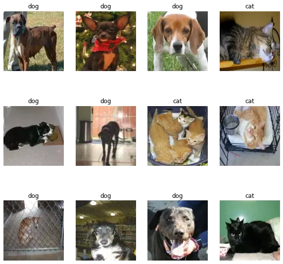
Build an Input Pipeline
We can use the tf.data.Dataset API to apply transformations to the dataset before feeding the data to the model.
Our images have different sizes. We need to resize them to a fixed size of 150×150 pixels.
We will also apply caching, shuffling, batching, and prefetching to speed loading. Shuffling the data is only necessary for the training and the validation set.
To learn more about creating input pipelines, please see how to load a dataset with an end-to-end example.
def create_dataset(ds, batch_size=32, buffer_size=1000, shuffle=True):
    ds = ds.map(
            lambda x, y: (tf.image.resize(x, img_size), y),
            num_parallel_calls=tf.data.AUTOTUNE
        )
    ds = ds.cache() # cache before shuffling for a better performance.
    if shuffle:
        ds = ds.shuffle(buffer_size, seed=42)
    # batch after shuffling to get unique batches at each epoch
    ds = ds.batch(batch_size)
    return ds.prefetch(1)

train_set = create_dataset(train_set, shuffle=True)
valid_set = create_dataset(valid_set)
test_set = create_dataset(test_set)
Let’s take a look at a batch of images and labels:
images, labels = next(iter(train_set))
print(images.shape)
print(labels.shape)
>>> (32, 150, 150, 3)
>>> (32,)
As you can see a batch contains 32 images and the images are resized to 150×150 pixels.
Data Augmentation
We generally use transfer learning when we have a small dataset, so it is good practice to apply data augmentation to artificially augment the dataset and thus get better accuracy and reduce overfitting.
Let’s create a Sequential model with some layers that will apply random transformations to the training set:
data_augmentation = tf.keras.Sequential([
    layers.RandomFlip('horizontal'),
    layers.RandomRotation(0.1),
    layers.RandomZoom(0.1),
])
Let’s see what an image will look like after applying these transformations:
# take an image from the batch
image = images[3]

plt.figure(figsize=(10, 10))
for i in range(9):
    plt.subplot(3, 3, i + 1)
    augmented_image = data_augmentation(image)
    plt.imshow(augmented_image / 255)
    plt.axis("off")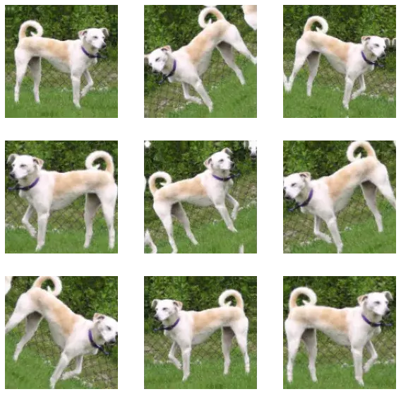
Feature Extraction
Convolutional neural networks are made of two parts: the first part consists of a stack of altered convolutional and pooling layers, which is generally called a convolutional base, and the second part consists of a densely connected classifier added on top of the convolutional base.
Here, we are going to use the VGG19 model as our convolutional base for feature extraction, then we will add a new densely connected classifier on top of the pre-trained VGG19 model to train it on the extracted features.
Load a Pretrained Model
Let’s start by loading the VGG19 model:
# load the pretrained model
base_model = tf.keras.applications.VGG19(
        input_shape=(150, 150, 3),
        include_top=False,
        weights="imagenet",
)
By using weights="imagenet", we are telling Keras to load the model with weights trained on the ImageNet dataset.
The include_top=False means that we load the model without the “second part” of the model; the densely connected classifier. We will add our own classifier as we said above.
We finally use the input_shape argument to specify the shape of the images that we’ll feed to the network.
Freeze the Base Model
In order to not lose the representations learned by the convolutional base (the VGG19 model), it is important to freeze its layers. Freezing a layer means that we make its weights non-trainable and thus gradient descent won’t update them.
This step needs to be done before compiling the model.
To freeze all layers of a model, we can set its trainable attribute to False:
# freeze all layers of the model
base_model.trainable = False
Add a FC Head on Top
Now let’s add a simple fully connected classifier using the Sequential model:
model = tf.keras.Sequential([
    tf.keras.Input(shape=(150, 150, 3)),
    data_augmentation,
    layers.Rescaling(scale=1.0/255), # rescale the pixel values to the [0, 1] range
    base_model,
    # add a new FC classifier on top of the base model
    layers.Flatten(),
    layers.Dense(256, activation='relu'),
    layers.Dense(1, activation='sigmoid'),
])
We first add the data_augmentation model, then a Rescaling layer is added to standardize the values to [0, 1] range, followed by the convolutional base, and finally, we add a new fully connected classifier.
Note that we are using a Dense layer with one node as our output. And since we are dealing with a binary problem, we used the sigmoid activation function.
Compile and Train the Model
Now that the convolutional base is frozen, we can compile and start training:
# compile and start training after freezing the layers
learning_rate = 1e-4
model.compile(loss='binary_crossentropy',
              optimizer=tf.keras.optimizers.RMSprop(learning_rate=learning_rate),
              metrics=['acc']
             )

epochs = 10
history = model.fit(train_set, epochs=epochs,
                   validation_data=valid_set)
Since there are only two classes, cats and dogs, we used the “binary_crossentropy” for the loss function. For multi-class classification, we would use the “sparse_categorical_crossentropy” loss.
Please note that training will be very slow. You will need a GPU to train the network. You can run the notebook of this tutorial in Colab or Kaggle and activate the GPU (it’s free!).
Epoch 1/20
364/364 [==============================] - 39s 80ms/step - loss: 0.4447 - acc: 0.7902 - val_loss: 0.5197 - val_acc: 0.7570
Epoch 2/10
364/364 [==============================] - 27s 73ms/step - loss: 0.3566 - acc: 0.8389 - val_loss: 0.3662 - val_acc: 0.8392
...
Epoch 8/10
364/364 [==============================] - 24s 66ms/step - loss: 0.2816 - acc: 0.8767 - val_loss: 0.2708 - val_acc: 0.8860
Epoch 9/10
364/364 [==============================] - 24s 65ms/step - loss: 0.2813 - acc: 0.8791 - val_loss: 0.3133 - val_acc: 0.8688
Epoch 10/10
364/364 [==============================] - 24s 65ms/step - loss: 0.2734 - acc: 0.8818 - val_loss: 0.3099 - val_acc: 0.8707
Learning Curves
Let’s plot the learning curves for the accuracy and the loss:
def plot_learning_curves():
    acc = history.history['acc']
    val_acc = history.history['val_acc']

    loss = history.history['loss']
    val_loss = history.history['val_loss']

    plt.figure(figsize=(10, 7))
    plt.plot(range(epochs), acc, "b", label="Training Accuracy")
    plt.plot(range(epochs), val_acc, "r", label="Validation Accuracy")
    plt.legend()

    plt.plot(range(epochs), loss, "g", label="Training Loss")
    plt.plot(range(epochs), val_loss, "orange", label="Validation Loss")
    plt.legend()
    plt.grid(True)

    plt.show()

plot_learning_curves()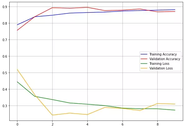
We reached an accuracy of 87% and thanks to data augmentation, the model is not overfitting the data. Nice!
Fine-tuning
Now what we can do to further improve the accuracy of the model is to use fine-tuning. Like we said before fine-tuning consists of unfreezing the top layers of the convolutional base and retrain the network with a low learning rate.
It is important to only try fine-tuning after training the densely connected classifier that has been added on top of the convolutional base because otherwise the updates of the weights will be too large and this will destroy the features learned by the layers being fine-tuned.
# we start by unfreezing all layers of the base model
base_model.trainable = True

# Freeze all layers except the 10 last layers
for layer in base_model.layers[:-10]:
    layer.trainable = False

# compile and retrain with a low learning rate
low_lr = learning_rate / 10
model.compile(loss='binary_crossentropy',
              optimizer=tf.keras.optimizers.RMSprop(learning_rate=low_lr),
              metrics=['acc']
)

epochs = 10
history = model.fit(train_set, epochs=epochs,
                    validation_data=valid_set)
Here we have unfrozen the 10 last layers for fine-tuning but you can try freezing/unfreezing more layers to see what performance you get. For example, I tried to unfreeze just the 5 last layers but the accuracy didn’t exceed 93%.
Epoch 1/10
364/364 [==============================] - 38s 98ms/step - loss: 0.2273 - acc: 0.9016 - val_loss: 0.1519 - val_acc: 0.9377
Epoch 2/10
364/364 [==============================] - 35s 97ms/step - loss: 0.1549 - acc: 0.9365 - val_loss: 0.1518 - val_acc: 0.9477
...
Epoch 8/10
364/364 [==============================] - 35s 97ms/step - loss: 0.0672 - acc: 0.9763 - val_loss: 0.1822 - val_acc: 0.9601
Epoch 9/10
364/364 [==============================] - 35s 97ms/step - loss: 0.0508 - acc: 0.9803 - val_loss: 0.1542 - val_acc: 0.9620
Epoch 10/10
364/364 [==============================] - 35s 97ms/step - loss: 0.0505 - acc: 0.9822 - val_loss: 0.1942 - val_acc: 0.9580
Let’s use the same code as before to plot the learning curves:
plot_learning_curves()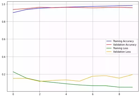
The model took longer to train, but it reached an accuracy of around 96% on the validation set. We get an improvement of 9%.
Evaluate the Model on the Test Set
import numpy as np

test_loss, test_acc = model.evaluate(test_set)
print(np.round(test_acc * 100, 2), '%')
>>> 182/182 [==============================] - 10s 49ms/step - loss: 0.1620 - acc: 0.9613
>>> 96.13 %
Let’s use the model to make some predictions on a batch of images:
image_batch, label_batch = next(iter(test_set))
proba = model.predict(image_batch)
# returns 0 if the probability of the prediction
# is below 0.5, otherwise it returns 1
y_preds = tf.where(proba < 0.5, 0, 1)


def show_prediction(image, y_pred):
    plt.imshow(image / 255)
    plt.title(class_names[y_pred.numpy()[0]])
    plt.axis("off")


plt.figure(figsize=(10, 10))
for i in range(12):
    plt.subplot(3, 4, i + 1)
    show_prediction(image_batch[i], y_preds[i])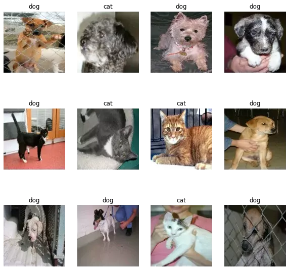
Further Reading
If you want to learn more about transfer learning and fine-tuning I recommend the following resources. I used all of these resources and more to write this article.
Books
- Part 2 Chapter 5 from the book Deep Learning with Python.
Articles
- Transfer learning and fine-tuning tutorial from the TensorFlow platform.
- Transfer learning and fine-tuning guide from the TensorFlow platform.
- Transfer Learning with Keras and Deep Learning.
Summary
In this tutorial, I showed you how to use transfer learning and fine-tuning with a pre-trained model to classify images from the dogs vs cats dataset.
For the feature extraction part we did the following steps:
- We started by loading the VGG19 model with weights pre-trained on ImageNet.
- Removed the fully connected layers (using the argument include_top=False) and replace them with new ones.
- Froze the convolutional base.
- Trained the new fully connected layers that was added on top.
This has given us an accuracy of 87% on the validation set. Then we tried to fine-tune the network by following these steps:
- Unfreeze the 10 last layers of the convolutional base.
- Trained the model with a low learning rate.
This allowed us to improve the accuracy of the model up to 96%.